Fundamentally, I study "cross low-rank matrix approximations". Let me unpack it for you.
Firstly, I'll shamelessly call any 2D array (table) of numbers a matrix. Obviously, one should also add how to work with matrices, i.e., what operations are allowed. And, one of the most important for us will be matrix multiplication (wiki). I will assume you already know how it works (otherwise please look it up). So, why is it important? As one can see from the definition, if, let's say, we have $M \times N$ matrix, then we can try to write it as a product of $M \times r$ and $r \times N$ matrices (see below).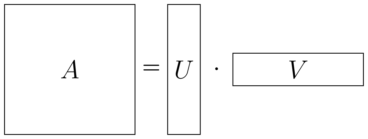 If we were to find this "decomposition" with small $r$, then we call it a "low-rank" (lowest $r$ is called "rank") factorization of our matrix $A$. And, in case this equality is not exact, we can call it a "low-rank approximation". You should already see why that's advantageous: we could have a huge matrix $A$, but the "factors" $U$ and $V$ are quite slim. As a result, we not only save on memory, but also on any operation cost, involving the factors.
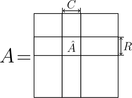
Now, how do we get these factors $U$ and $V$? That is where the "cross" method comes into play. Turns out, there is an easy way to select the factors: one can use $U = C$ and $V = \hat A^{-1} R$, where $C$ are some columns of $A$, $R$ are some rows and $\hat A^{-1}$ is the inverse of the submatrix at their intersection (remember that picture in the beginning? Let me show it again on the right).
If the factorization is exact, then there is no problem here. However, if it is not, the error heavily depends on the rows and columns we select. It turns out, it is a good idea to search for the submatrix $\hat A$ (and thus its rows $R$ and columns $C$) with large volume (absolute value of the "determinant"). That's what was already known before I even started my bachelor's degree.
So, what was I doing? Previously I considered the number of rows and columns equal to the approximation rank $r$. But what if we can select more? Is there a relatively simple way to improve our approximation without increasing its rank?
![]()
And there is. To do that, instead of searching for the submatrix with the large volume, one should search for the submatrix with the large "projective volume" (product of the first $r$ of its singular values) and do pseudoinverse, keeping only the first $r$ singular values nonzero using singular value decomposition (wiki). That "keeping the first $r$ singular values" is denoted by subscript $r$ and is going to be my unseen (because of how small it is) website's icon.
Since we only modify the small submatrix $\hat A$ it is not very costly, but allows to quickly get arbitrarily close to the optimal approximation in Frobenius (euclidean) norm. In my papers, I show that it indeed (usually) works and how to quickly find this submatrix with the large projective volume.
Here I'll need to be a little bit technical, please bear with me.
Aggregation in granular gases (and any other system) is described by Smoluchowski equations
$$ \frac{dn_k}{dt} = \frac{1}{2} \mathop{ \sum}\limits_{i+j=k} C_{ij} n_i n_j - \mathop{ \sum}\limits_j C_{kj} n_k n_j.$$
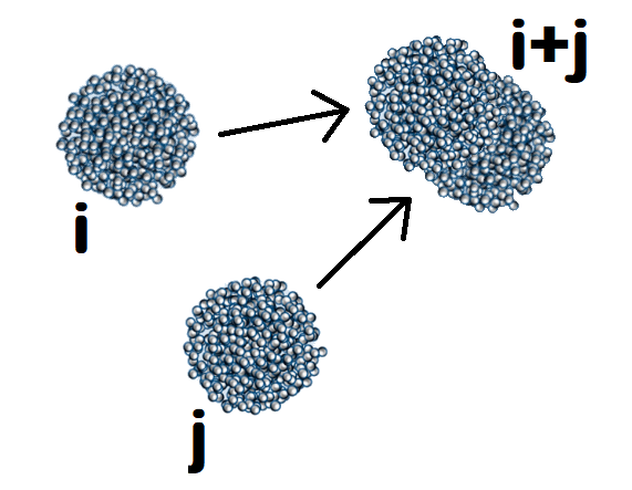
Each one is a differential equation, i. e., it describes the rate of change of the concentrations (also called number densities) $n_k$ of size $k$ clusters. In this simple case $k$ is just an integer, describing the relative size of the cluster. On the right, we count all of the collisions, using the rates $C_{ij}$. For example, the number of collisions between the clusters of size $i$ and $j$ is proportional to the number of clusters of size $i$, $n_i$, times the number of clusters of size $j$, $n_j$, times how often they collide, which we denote by $C_{ij}$. We devide by $2$ because we count $(i,j)$ and $(j,i)$, and it's the same pair. So, that's how many clusters of size $k = i + j$ appear, this is the first term in the right-hand-side. But, clusters of size $k$ also can aggregate to form even larger clusters, so we also subtract aggregation in all possible pairs $(k,j)$, which is the second term.
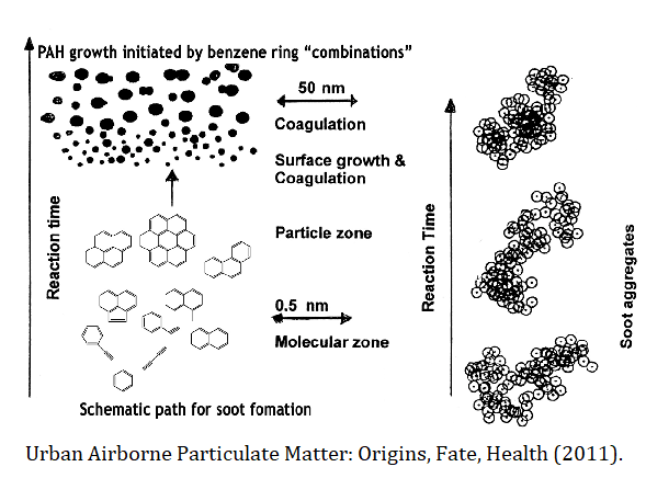
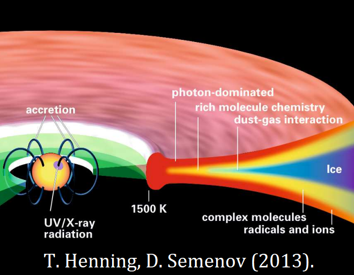
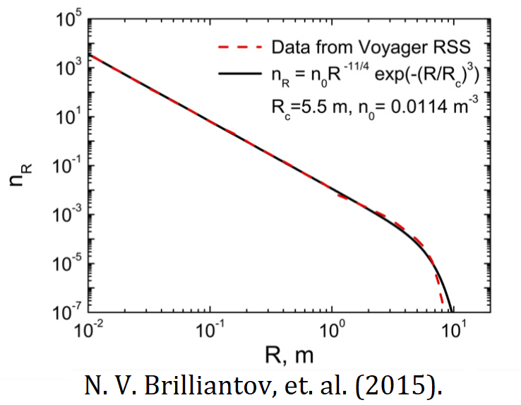
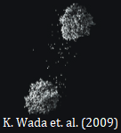
Now, as mentioned before, this is an infinite system (there are infinitely many possible sizes $k$). In practice, when we limit ourselves to a finite number sizes, this number can still be about a million, if we want to describe our gas accurately. For example, dust particles in protoplanetary rings (see figure below) can be between micrometers and centimeters, so their masses span a dozen orders of magnitude.
Fortunately, there are fast low-rank methods to solve Smoluchowski equations, developed by Sergey Matveev. I have also improved these methods, so that they would work for the case, when the rates $C_{ij}$ change in time.
However, there is another way to bypass the solution of these complex equations altogether. To do that, one can perform Monte Carlo simulations. One first creates some finite system of numerical particles, estimates, how often they collide with each other and performs these collisions. As the number of particles decreases because of aggregation, one just adds more of them. This idea can be used to simulate any gases (without aggregation too) and see, how many particles are there with each speed. So yeah, if we can just simulate the collisions instead of solving the equations, then what's the problem?
The problem is, how can we decide who collides when? "Well," – you can say, – "we have our collision rates $C_{ij}$ (or whatever analogue in case we do not have aggregation). Just select particles according to them. Higher rate - higher chance of selecting this particular pair." And that's great. But. If we have $N$ sizes, then there are $N \cdot N$ pairs. Do we need to check all of them? EVERY time we need to collide just two particles? And remember, they also need to be updated, as the speeds (and, possibly, numbers) of particles change after each collision. That's too much.
Luckily, there is a way to do that significantly faster (in $O \left( \log N \right)$ time, i. e., the complexity is logarithmic in the number of sizes). And it works for ANY Monte-Carlo simulations: whether you want to solve Smoluchowski equations or just simulate some mixture of gases with many different sizes. Although it is also based on the low-rank decomposition, one does NOT need $C_{ij}$ to be low-rank: just to be bounded by a low-rank kernel (which worked for every example I know of, even some exotic ones like aggregation of rectangles).
Unfortunately, I can't talk about it in detail, since I am still working on the paper. But, again, you can find some of the ideas here.
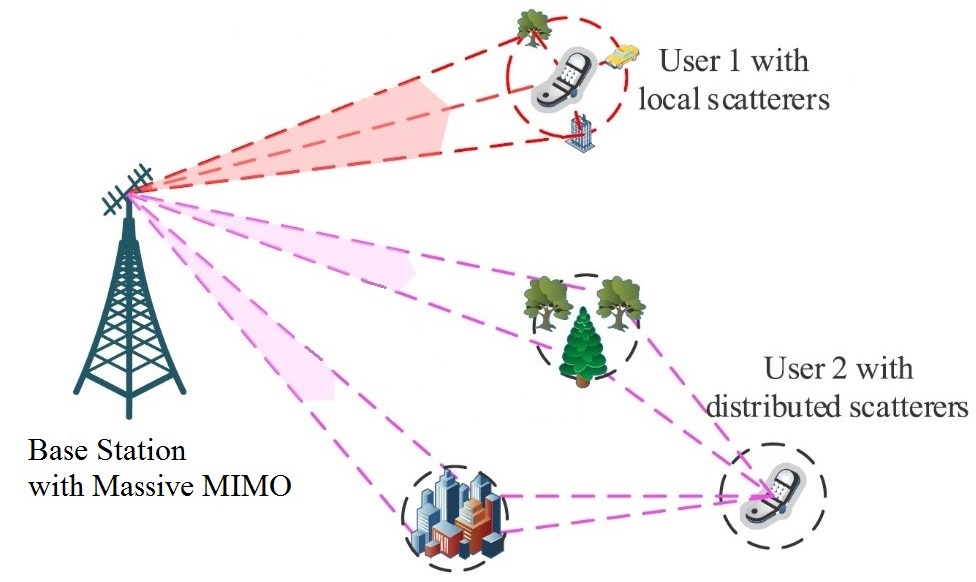
Since I mostly worked on the problem of channel estimation, let us discuss it in more detail.
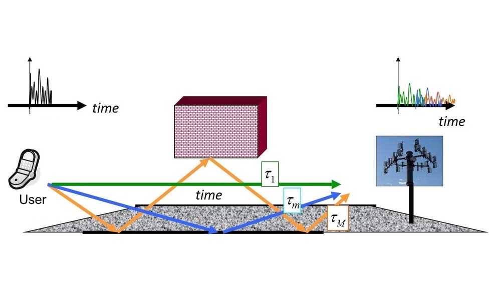
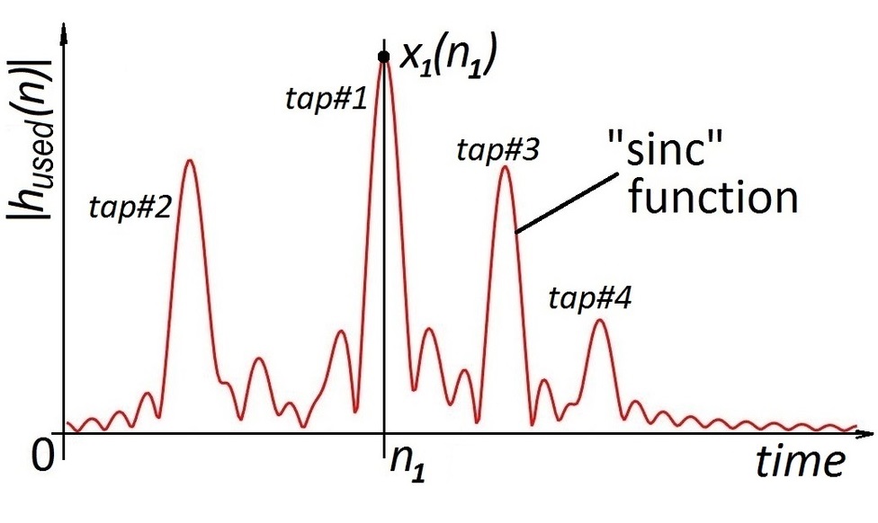
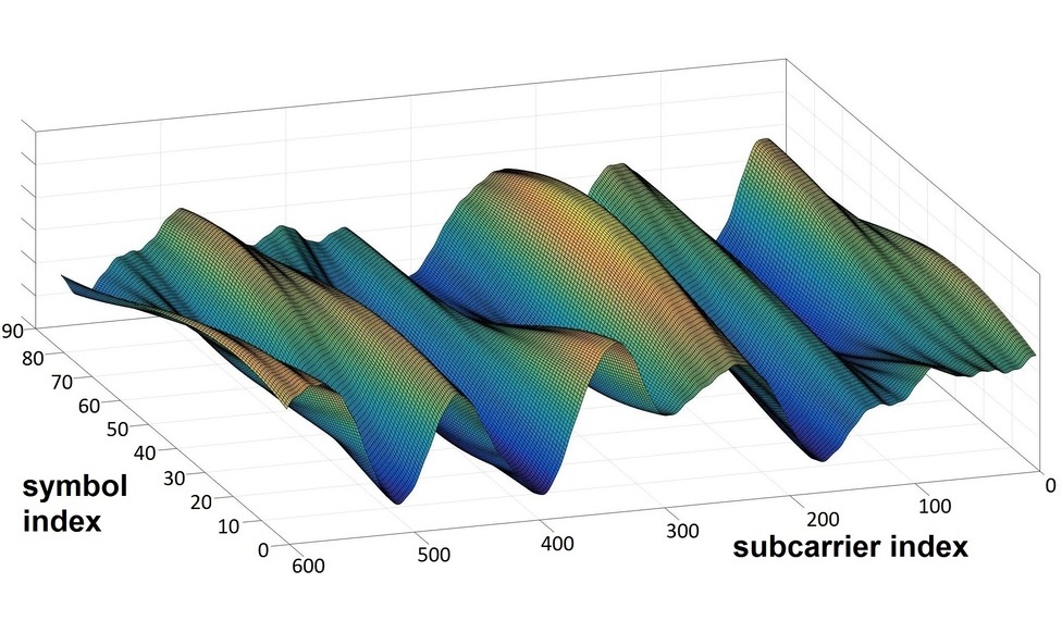
Channel estimation is the process, where you send a known signal (called a pilot) to find out, what the received signal would look like. Ideally, we want to catch all sources of the reflected (non-line-of-sight) signals, which correspond to the peaks below. This peaks are smoothed out, because of the technique called "oversampling": in practice, the signal is not measured continuously, but only at certain points of time. This technique allows to find the exact point of time the signal came more accurately at the cost of turning the discrete peaks into "sinc" functions. The examples of (noiseless) received signals using this technique are shown below:
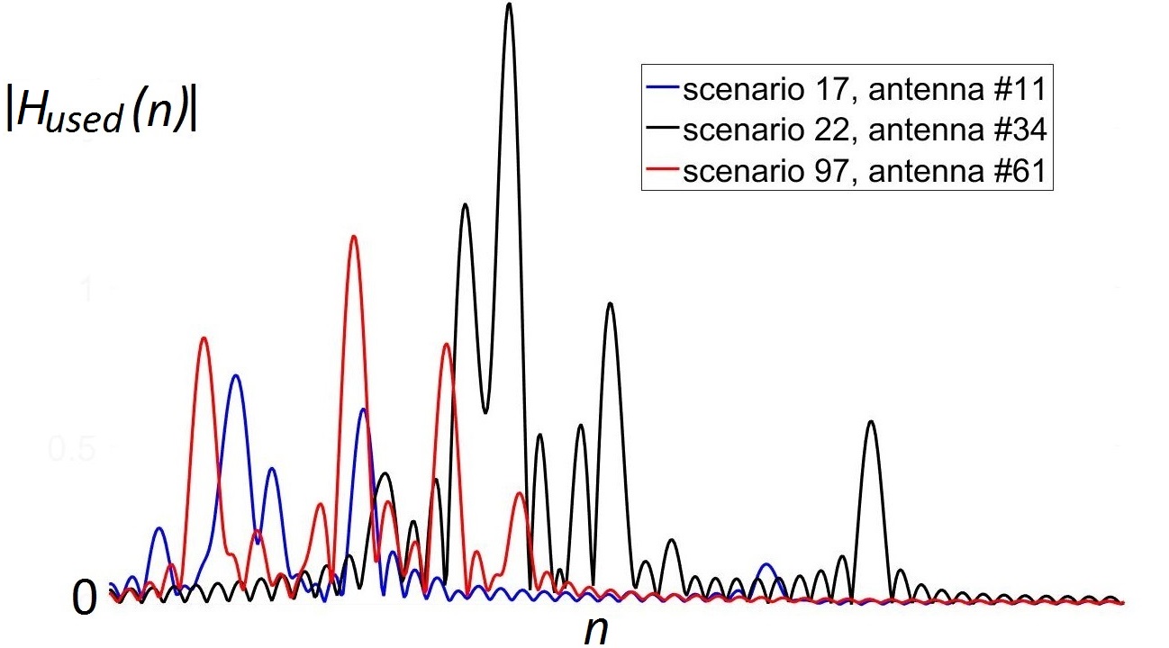
The idea of our method is to find the maximums and place the "sinc" functions there. If we do it for all the maximums, we are great, and the signal is restored almost exactly.
Now, the problem is, which maximums to keep? In practice the noise level is almost the same as the signal power. So, the question arises: which maximums are the actual signal peaks and not just some random bursts of noise?
The idea at the base of all of our algorithms is actually quite simple, which, in my opinion, makes it quite beautiful. Firstly, we only select the peaks, which have the total power $\| y \|^2$ greater than the average noise power $\sigma^2$. It turns out, that is actually almost exactly optimal. IF we do one more thing.
Namely, the selected peaks (we select them iteratively) are rescaled by the factor $1 - \frac{\sigma^2}{\| y \|^2}$. If you are familiar with the Minimum Mean Square Estimate, which produces the factor $\frac{1}{1 + \frac{\sigma^2}{\| x \|^2}}$, you can see the similarities. In fact, it is exactly the same estimate: $\| x \|^2$ is the expected (noiseless) signal power, so you can just add noise $\| y \|^2 = \| x \|^2 + \sigma^2$ and get the factor we use!
"But wait!" – some of you who are too knowledgable in the probability theory might say, – "Minimum Mean Square Estimate is only applicable if you know the variance (expected signal power in our case). And you do not know it! It can't be estimated just from one sample! You should have used the unbiased estimate instead." And you would be right. Formally. Except, I claim that the power CAN be estimated just from one sample and, moreover, this rescale is, in a certain way, the best one and works in every scenario we had.
In my opinion, this result is a strong evidence towards Bayesian understanding of probability: it does not use any proior samples to estimate the a-priory distributions, yet, somehow, uses them. And, naturally, this approach can be used in many areas as an easy and effective replacement of the unbiased estimate.
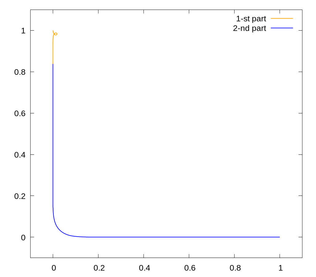
This is the shortest path from $(1,0)$ to $(0,1)$, such that $\int xy \, dx \, dy = 0$ under the curve. The length is approximately $1.9881$.
The difficulty here is that this problem can't be solved just by using the "shooting method", and even Pontryagin's maximum principle does not help.
Nevertheless, I have found a way to solve such problems and even published a code for this particular case.
Gold medal from Russian Academy of Sciences
Apart from my master's thesis being awarded a gold medal, I also received a couple of winner diplomas at MIPT conferences, while studying there.